Mini Guide for Basic Commands in the XXX Program

Sébastien Masson `< Sebastien.Masson_at_locean-ipsl.upmc.fr>`

Albert Fisher

Françoise Pinsard `<Francoise.Pinsard_at_locean-ipsl.upmc.fr>`

Steve Navarro

svn Id of xml source file : $Id: mini_notice.xml 157 2006-08-21 09:01:50Z navarro $

Revision History
Revision 0.0	May 29, 2000
French release by Sébastien Masson
Revision 0.1	July, 2002
Translation by Albert Fisher
Revision 0.2	July 20, 2006
HTML to XML/Docbook migration by Françoise Pinsard

Table of Contents

1. XXX widget functions

1.1. Launching XXX
1.2. Description of XXX window

2. Mouse Actions

2.1. In the graphics window on a horizontal plot
2.2. Create multiple plots on the same sheet and make them interact

3. What should I do when it breakdown

1. XXX widget functions

1.1. Launching XXX

The first command to type is

idl> @init

Afterwards, to work directly with XXX, type:


idl> xxx

A window will open with 2 lines to complete.

Figure 1. Window xxx 1

	Data file
	Init method
	Init program

1.1.1. File name

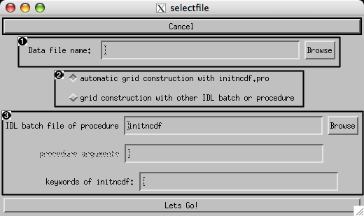
the name of the data file. The name can be typed directly in the window provided, or selected with the help of the browse button.

1.1.2. Grid initalization method

By default, "automatic grid construction with initncdf.pro" is checked.

But you can choose an other grid by checking "grid construction with other IDL batch or procedure"

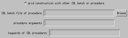
1.1.3. Grid initalization parameters

Figure 2. Window xxx 1

the second the name of the initgrid.pro script which will permit the reading and processing of the grid associated with the data file.

Once these two lines have been completed, click on let's go.

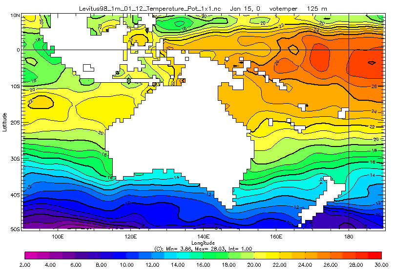
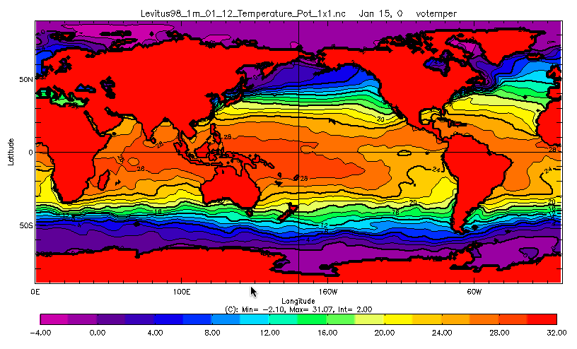
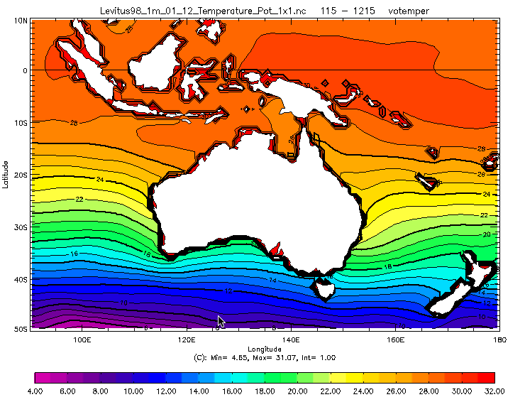
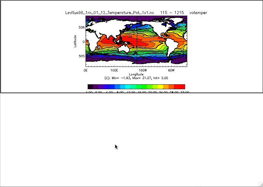
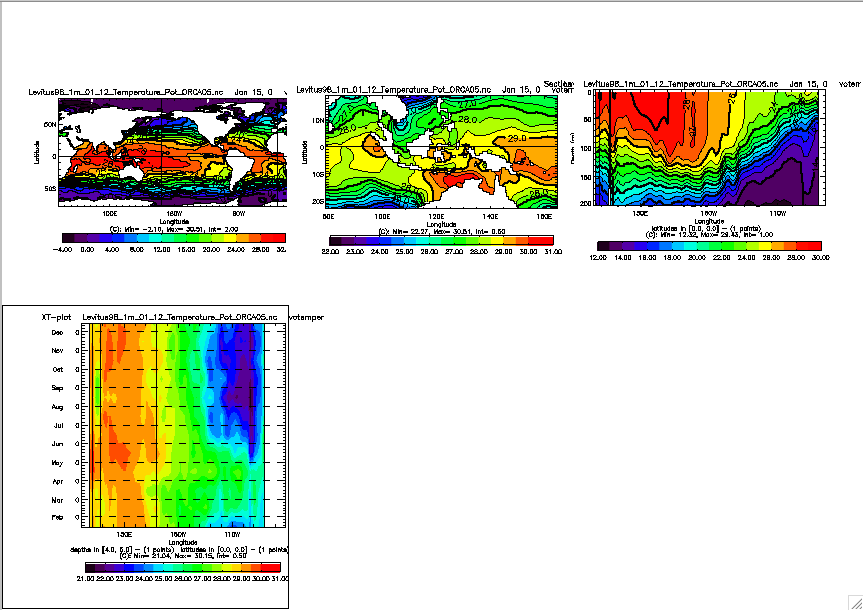
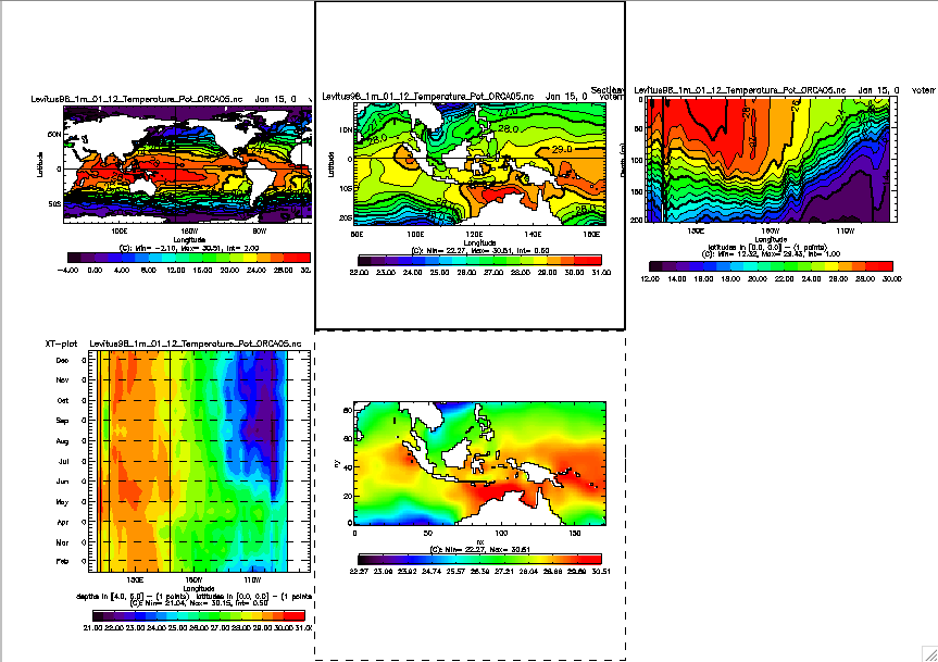
For example, we choose the mask "tst_initlev". Compare the result with "automatic grid construction with initncdf.pro" checked. Cf Figure 23, “Oceania at 125 metters of depth without a mask”

Figure 3. Oceania at 125 metters of depth with a mask

1.2. Description of XXX window

Now the XXX window will open.

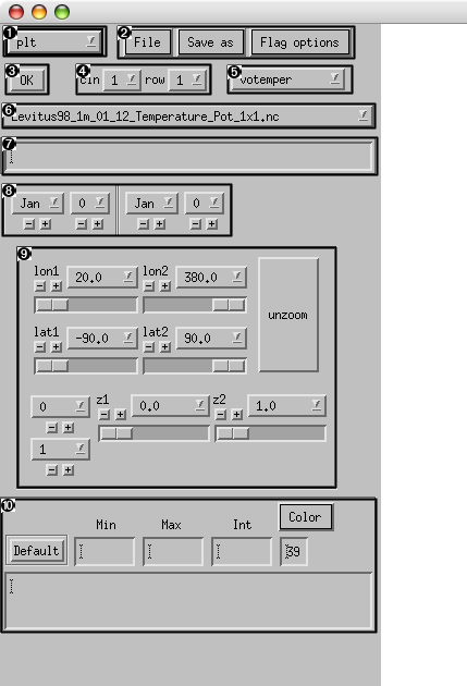
Figure 4. Window xxx 2

	Plot type
	Menu
	OK
	Page layout
	Variables list
	Files list
	Command text
	Calendar
	Domdef
	Spefications

It's configuration will change depending on whether you are in portrait or in landscape, but here are the different parts available for your use.

1.2.1. Plot type list

allows specification of the type of plot desired.

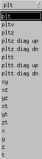
Figure 5. Differents plot types avaibles

Note

If the type plt is selected, the selection of plot type is made by mouse. Cf Section 2.1, “In the graphics window on a horizontal plot”

1.2.2. The menu bar made up of 3 submenus

1.2.2.1. File submenu

Figure 6. The File menu

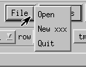
Open: to open a second file. Same procedure as during the launching of XXX. The new file can be on a different grid, with different variables, with a different time base.
New XXX: to open a second XXX window identical to the first.
Quit: to close the XXX window.

1.2.2.2. Save As submenu

Figure 7. The Save As menu

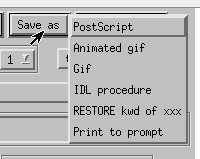
Postscript: to save in Postscript format
Animated gif:to create an animation from the XXX window. Careful, the creation of an animation is only possible if none of the plots have a time axis, and if the plots are all on the same time base (calendar). On the other hand, animations of horizontal and vertical plots, with different color palettes (for those not on an X-terminal), are possible.

Note

the creation of animations has a tendency to saturate the video memory of X-terminals, crashing the entire program...
Gif: to save a gif of the XXX graphics window.
IDL procedure: to save the command history that has created the plot. For example if I save the commands in xxx_figure.pro, I can then launch a new IDL session and type:
```
idl> @init
idl> xxx_figure
```
and I'll obtain the saved figure.
```
idl> xxx_figure,/post 
```
or
```
idl> @ps
```
will then create a Postscript file of the figure.
RESTORE kwd of xxx:
Print to prompt: lists in the IDL window the command history that created the last plot. Useful primarily for debugging...

Test the various possibilities in the Save As menu.

1.2.2.3. Flag options submenu

Figure 8. The Flag Option menu

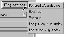
Portrait/Landscape: changes the configuration of the plot.
Overlay: to plot contours of a different field on top the one represented as color-filled contours. It is necessary to relaunch the entire plot to make this work!
Vecteur: to plot a vector field on top of contours. Only works on horizontal plots (plt.pro). As for Overlay, a relaunch of the entire plot is necessary.
Longitude / x index: switches longitude labelling of the plot subdomain from degrees to indices following i.
Latitude / y index: switches latitude labelling of the plot subdomain from degrees to indices following j.

Test the various possibilities in the Flag options menu.

Caution

Careful, a selected option remains selected until it is reclicked.

1.2.3. OK button

click on this OK button is required to make a new plot appear

1.2.4. Page Layout

specify the number of columns and rows for plots on the sheet of paper.

Figure 9. Number of Column

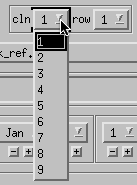
For example: For 2 cln and 2 row. For explanations, see further.

Figure 10. A frame with several graphics

1.2.5. List of variables

you can choose the variable to work on.

Figure 11. differents Variables avaible

1.2.6. List of open files

you can choose the file to work on.

Figure 12. List of open files

1.2.7. Command text

To specify the computation you want to do. Examples:

1.2.7.1. Without any Command Text

Figure 13. Graphic by default

1.2.7.2. With the command text /realcont

Figure 14. Command text area

Figure 15. Graphic with the command text "/realcont"

1.2.7.3. With the command text /realcont+ map=[90,0,0]+ /ortho+ cell_fill=2.

Figure 16. Command text area with the right syntax

Figure 17. Polar Projection

Note

In the default case, the name given to a field is of no importance.

1.2.8. Calendar

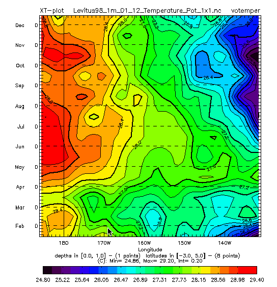
The calendar is made up of two droplists, which allow specification of two dates, the beginning and end of a time series, or the period over which to average before plotting.

Example: The first plot is during January.

The second plot is from January to December.

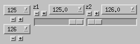
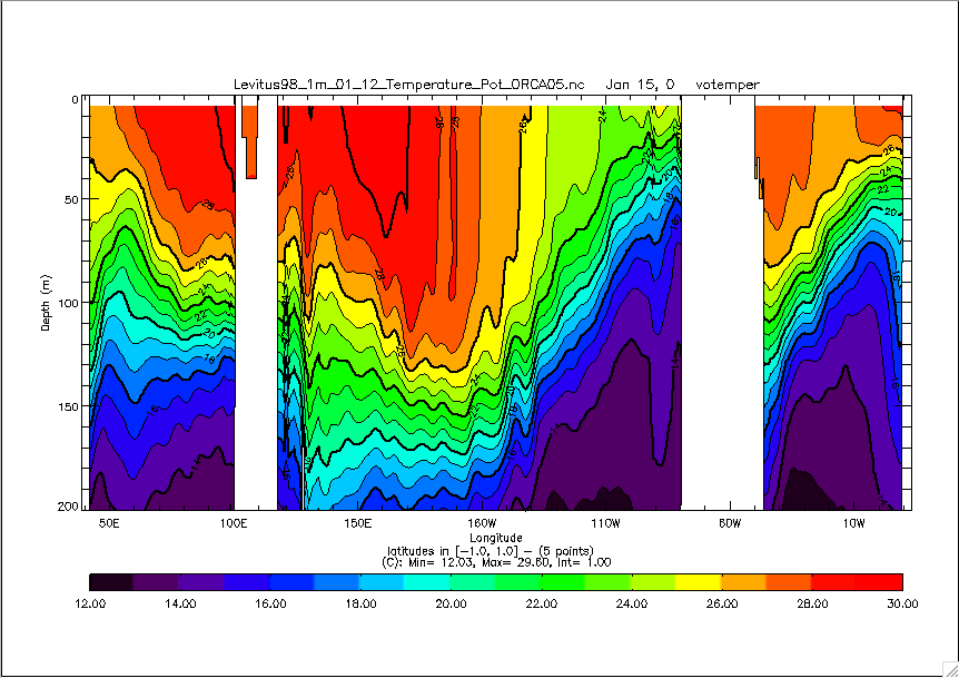
Figure 18. Graphic with 2 different period of study

1.2.9. Define the domain

A series of widgets that allow specification of the min/max limits of the domain in longitude/x-index, latitude/y-index, and depth in levels or meters. For depth, one can specify in levels for a horizontal plot, and in meters for a vertical plot.

1.2.9.1. Without any domain specification

Figure 19. Domain by default

1.2.9.2. With a zoom on Oceania

We can zoom, between 0 and 1 meter of depth, on the Oceania, by playing with the part Domdef, with this configuration

Figure 20. Change Domain area

This configuration give us:

Figure 21. Graphic with a specified domain

1.2.1. With the specification of the depth

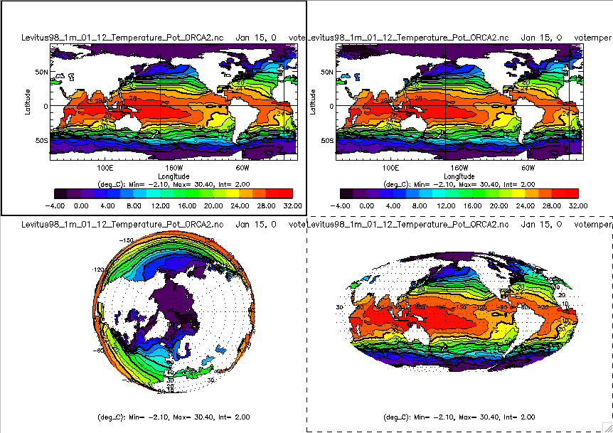
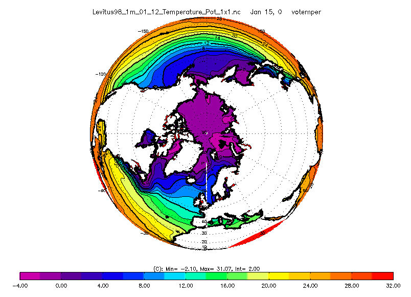
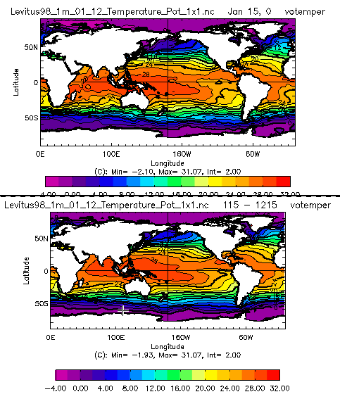
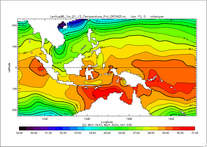
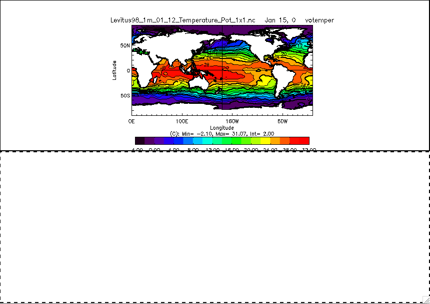
If we want to see the temperature of the ocean between 125 and 126 meters of depth

Figure 22. Change depth area

Figure 23. Oceania at 125 metters of depth without a mask

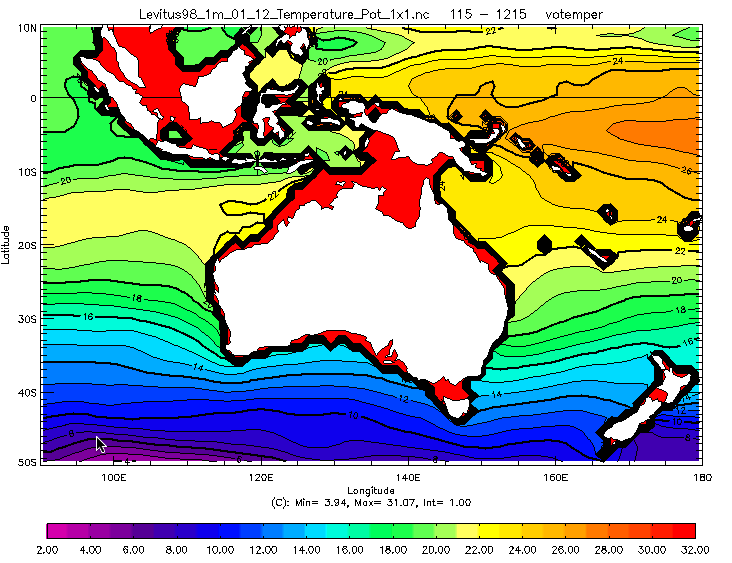
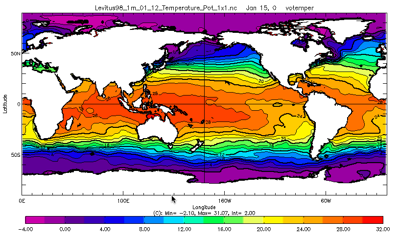
As you can see, at this depth, we can see the difference between the continent at the surface and the real goegraphy of the terrain. If we want to see only the terrain at the specified depth, we have to put a mask. Cf Figure 3, “Oceania at 125 metters of depth with a mask”

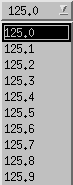
You can define precisely the depth you want to see:

Figure 24. The Precise Depth menu

1.2.10. specify your plot

1.2.10.1. Specify the min, the max and the interval

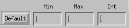
You can specify the min, max, and contour interval by filling out the provided boxes!

You can restore configuration by default by pressing the "default" button.

Figure 25. Specification area

1.2.10.2. Specify the palette to be used

For the color palette, you can either specify the name or go search for one among the palettes available.

Figure 26. The Color menu

The "keywords" window allows specification of all desired keywords. These keywords can be those of plt.pro, pltt.pro, pltz.pro, plt1d.pro, or those of contour, plot, or all other programs that are used. Cf Section 1.2.7, “Command text”

2. Mouse Actions

2.1. In the graphics window on a horizontal plot

Select a domain and select the horizontal plot (plt), vertical plot (pltz), or the hovmoeller plot (pltt):

The domain we'd like to select for the plot is determined by one of its diagonals, defined therefore by two points. The first point is defined when the mouse button is pushed, then the mouse is moved, and the second point is defined as the mouse button is released (click-drag). The domains are thus defined by a long click (LC). To determine which type of plot should be made of selection, use:

If the plot selector is on plt

the left mouse button to create horizontal plots (plt)
the middle mouse button to create vertical plots (pltz)
the right mouse button to create common hovmoellers for xt and yt cuts (pltt)

In summary:

Figure 27. LCL--->plt

Figure 28. Horizontal Plot
Figure 29. LCM--->pltz

Figure 30. Vertical Plot
Figure 31. LCR--->pltt

Figure 32. Common hovmoeller for xt and yt cuts

Note

If the plot selector is on something other than plt the indicated plot type is made.

2.2. Create multiple plots on the same sheet and make them interact

Select the number of columns and rows for the page.

Create a first plot. It will appear in the first frame.

To create a plot in another frame double-click in the frame with the middle button (DCM). A black dotted frame will surround the designated frame, the “target” frame. A black frame will surround the first plot. This is the “reference” frame, in other words the one that all the XXX widgets refer to. Change for example the date and create a new plot. With a left button double-click in the first frame, all the widgets change and refer again to the first plot. A double-click with the right button in the second frame will erase the plot.

In summary:

Figure 33. DCL--->“reference” frame

Figure 34. The reference frame is selected
Figure 35. DCM--->“target” frame

Figure 36. The target frame is selected
Figure 37. DCR--->erase the frame

Here's a series of commands to show how this works.

Select a 3-D field and create 6 frames for the sheet of paper.
Create a horizontal plot in Frame 1
DCM in frame 2, LCL on the plot in frame 1, to create a horizontal zoom in frame 2.

DCM in frame 3, LCM on the plot in frame 1, to create a vertical cut in frame 3.

DCM in frame 4, LCR on the plot in frame 1, to create a hovmoeller in frame 4.

Figure 38. Frame with four plot

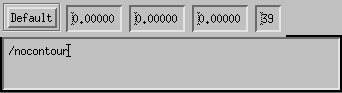
To redo the hovmoeller with the keyword

/nocontour

DCL in frame 4 which now becomes the reference and target frame.
Add the keyword

/nocontour

Figure 39. Command text area
click OK, and the plot is redone.

Figure 40. The fourth plot with the keyword "nocontour"

in frame 5, let's create the same plot as in frame 2 except with different dates

DCL on frame 2
DCM on frame 5
change the date
click on OK

Figure 41. Frame with five plot

3. What should I do when it breakdown

in the IDL window, type
```
idl> retall
```
DCR to erase the problem frame.
change the orientation of the plot by pressing Flag options -> Portrait/Landscape. Cf Section 1.2.2.3, “Flag options submenu”
quit XXX cleanly using quit from the File menu. Cf Section 1.2.2.1, “File submenu”

Note

Always avoid if at all possible closing and killing the XXX window, but rather select quit from the File menu. XXX uses a large number of pointers, and wantonly killing the window will leave a large number of unused variables in memory, which could in the end overflow. To clean up this memory:

idl> ptr_free, ptr_valid()